Loads - Distributed Loads

Distributed loads are loads that are spread across all or part of a member or wall panel and can be of uniform, stepped, or varying magnitude such as triangular or trapezoidal. You may define distributed loads graphically or by using the spreadsheets. See Drawing Distributed Loads below to learn how to draw distributed loads graphically.

Note

If a member has offsets defined, the offset distances will NOT be loaded. The locations are still relative to the I joint, but if the start location is less than the I End Offset, the part of the load applied along the offset distance will be ignored. The same is true for the end location and the J End Offset. So a full-length load is actually applied to a length equal to the full I to J joint distance minus the I-End and J-End offset distances.

Drawing Distributed Loads

You can apply distributed loads to members or wall panels. The direction of the load may either be defined in the global axes or the local axes of the member and may also be projected. For full length loads leave the Start and End Locations as zero.

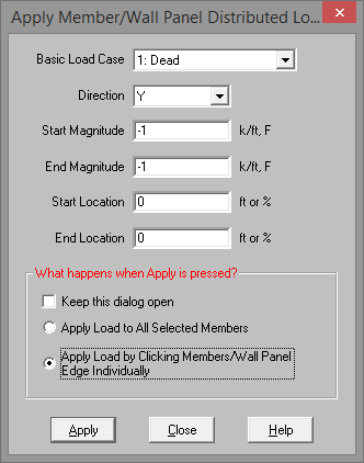
Make sure that you are careful to enter the correct Basic Load Case number that you want the loads assigned to.

To Apply Distributed Loads

If there is not a model view already open, then click on the RISA Toolbar to open a new view and click to turn on the Drawing Toolbar if it is not already displayed.
Click the Apply Distributed Load button and define the load.

For full member length loads leave the Start and End Locations as zero.

You may choose to apply the load to a single element at a time or to an entire selection of members and/or wall panels.

To apply the load to only a few members/wall panels, chooseApply Entry by Clicking Items Individually and click Apply. Click on the members/wall panels with the left mouse button to apply the load.
To apply the load to a selection of members/wall panels, choose Apply Entries to All Selected Items and click Apply. The load will then be applied to all the selected elements in the model.

Note

To apply more loads with different parameters, press CTRL + D to recall the Distributed Loads settings.
You may also specify or edit distributed loads in the Distributed Load Spreadsheet.

Distributed Loads Spreadsheet

The Member Distributed Load Spreadsheet records the distributed loads for the member elements and may be accessed by selecting Loads Distributed Loads on the Spreadsheets menu, or by clicking Distributed Loads on the Data Entry toolbar.

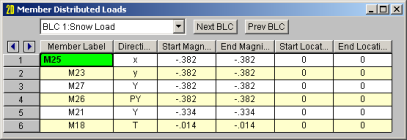
The first column contains the Label of the element being loaded.

The Direction specified in the second column indicates which axes are to be used to define the load directions and whether or not the load is to be projected. Directions are discussed in the next section.

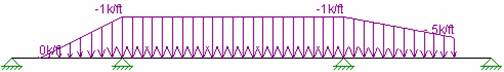
Start and End Magnitudes of the load must be specified. Start and End locations for the load need only be specified if the load is not across the full member length. If both locations are left as zero then the load will be applied across the full member length.

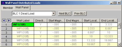
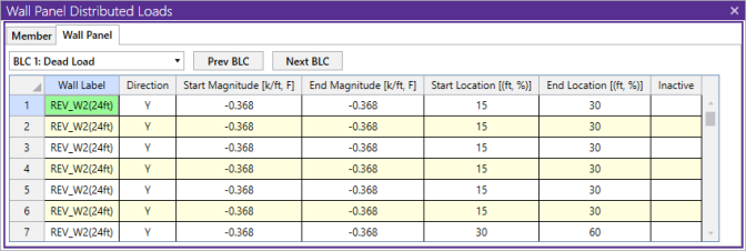
The Location columns contains the location of the load. The location is the distance from the I-joint of the member and is unaffected by any member offsets. The location of the load may be defined as a percentage of member length. To define the distance from the I-joint as a percentage of member length, enter the percentage value (0 to 100), preceded by the symbol "%". For example, a load starting or ending in the center of the member would be defined with a start or end location of "%50". Using a percentage value is handy if the member's length will be changing due to editing of the model coordinates and you wish to have the load some proportional distance from the I end.

The Wall Panel Distributed Loads Spreadsheet records the distributed loads on your wall panels. Note that the loads are specific to the BLCs and that you can use the drop-down list to choose a different one. The columns in the spreadsheet are the same as the member distributed load spreadsheet.

Distributed Load Directions

The direction code indicates how the distributed load is to be applied. Following are the valid entries:

Entry	Load Direction


x or y	Applied in the member’s local x or y-axis
X or Y	Applied in the global X or Y-axis

T (or t)	Thermal (temperature differential) load
PX	Projected load in the global X-axis direction
PY	Projected load in the global Y-axis direction
SX	Pressure load applied to projected surface of member in the global X-axis direction
SY	Pressure load applied to projected surface of member in the global Y-axis direction
Sy	Pressure load applied to projected surface of member in the local y-axis direction

This diagram illustrates the difference between local (x, y, z) and global (X, Y, Z) direction loads:

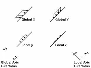
In this diagram, the local y and global Y loads shown are both negative, while the local x and global X loads are positive. As can be seen, local direction loads line up with the element's local axis directions, so their direction relative to the rest of the model changes if the member/wall panel orientation changes. Global loads have the same direction regardless of the element's orientation.

A distributed load in the Mx direction will be applied to the member/wall panel according to the right hand rule. Remember that the positive local x-axis extends from the I joint of a member towards the J joint.

Projected Loads

Keep in mind that global loads are applied without being modified for projection. For example, a full length Y direction load of 1 kip/foot applied to a 10 foot member inclined at 45 degrees generates a total force of 10 kips. Projected loads, on the other hand, are applied in the global directions but their actual magnitude is influenced by the member's orientation. The load is applied to the "projection" of the member perpendicular to the direction of the load. For example, a "PY" direction load is a projected load applied in the global Y direction. The actual magnitude of the load is the entered magnitudes reduced by the ratio L/Lx, where L is the member's full length and Lx is the member's projected length on the global Xaxis. See the following figure:

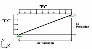
So the total load generated is equal to the input magnitudes applied along the projected length. This generated force is distributed along the full member length, so the applied magnitudes are reduced accordingly.

For additional advice on this topic, please see the RISA Tips & Tricks webpage at risa.com/post/support. Type in Search keywords: Projected Loads.

Surface Loads

This is a load type that applies a pressure load to the face of the member in the direction specified. If a local axis direction is specified then the load will be applied to the strong/weak direction of the member regardless of the member orientation. If using the global coordinates then the program will take the projected face of the element in the direction in question and calculate the pressure area accordingly.

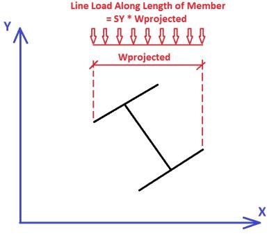
The program then takes this pressure multiplied by the width of the pressure area and creates a line load that is then applied to the member.

Note:

Distributed pressure loads can not be applied to tapered members or wall panels.